
This article appeared on Hacker News. Link to the discussion here!
A few weeks back, I implemented GPT-2 using WebGL and shaders (Github Repo) which made the front page of Hacker News. Here is a short write-up over what I learned about old-school general-purpose GPU programming over the course of this project!
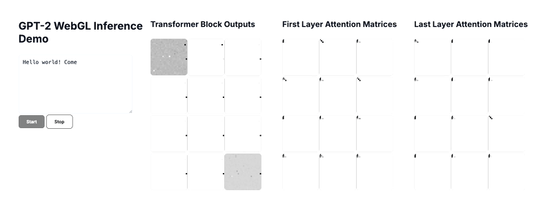
Above is a gif of the final demo, which you can run locally via the github repo above.
The Origins of General-Purpose GPU Programming#
In the early 2000s, NVIDIA introduced programmable shaders with the GeForce 3 (2001) and GeForce FX (2003). Instead of being limited to predetermined transformations and effects of earlier GPUs, developers were now given unprecedented control over the rendering pipeline, enabling much more sophisticated visual effects. These programmable shaders laid the foundation for modern GPU computing.
Researchers soon discovered that certain computations (like linear algebra involving matrices and vectors) could be accelerated by casting them as graphics operations on the GPU. However, using shader languages like OpenGL’s GLSL for no-graphics tasks was cumbersome. By the mid-2000s, the need for a more straightforward, non-graphics interface to GPUs had become clear, and NVIDIA saw a new opportunity.
Inspired by the demand for general-purpose GPU (GPGPU) programming, in November 2006, NVIDIA released CUDA, the Compute Unified Device Architecture. CUDA is a parallel computing platform and programming model that gives developers direct access to the GPU’s computational power without the intermediary of a graphics API. With CUDA, one could write C/C++ code to execute on the CPU using straightforward extensions for parallel kernels and managing GPU memory explicitly. This meant that developers could now ignore graphics-specific concepts and dramatically lowered the barrier for general-purpose GPU computing. Following CUDA came OpenCL which expanded general purpose computing beyond the NVIDIA ecosystem.
Graphics API vs Compute API#
Traditional graphics APIs like OpenGL are centered around a fixed-function pipeline tailored for rendering images. The pipeline consists of stages like vertex processing, rasterization, fragment processing, etc. Each stage can be programmable with shaders, but the overall flow is fixed. Using the OpenGL graphics pipeline to do general-purpose computation required a lot of boilerplate. One had to pack data into texture formats, use off-screen framebuffers to capture the results, and often perform multiple render passes to accomplish multi-stage algorithms.
In contrast, OpenCL and CUDA expose a direct compute model:
- Kernels, not shaders: You write a function and then launch thousands of copies to run in parallel (no notion of vertices or fragments).
- Raw buffers: Allocate arrays of floats or integers, read/write them directly, and move them back and forth between host and device with explicit copy calls.
- User-driven pipeline: You define exactly what happens and when instead of using a predefined fixed sequence of rendering stages.
The result is a far more natural fit for linear algebra, simulations, physics, ML, and any algorithm where you just want to compute independent calculations in bulk.
In OpenGL, the output would ultimately be pixels in a framebuffer or values in a texture; in OpenCL, the output can be data in any form (float arrays, computed lists of numbers, etc.) which you then transfer back to the CPU or use in further computations. This makes OpenCL more suitable for general algorithms where you just want the numerical results.
Implementing GPT-2 via Classic GPGPU Programming#
Instead of CUDA or OpenCL, I decided to implement the forward pass of GPT-2 using the old school way, using the graphics pipeline.
First, we need to cover textures, framebuffers, vertex and fragment shaders, and other graphics specific concepts needed for this.
Textures & Framebuffers: The Data Bus#
In traditional graphics rendering, a texture is simply a 2D (or 3D) array of pixel data stored in GPU memory. When you map a texture onto a triangle, the fragment shader “samples” it to look up color values. In our compute‐as‐graphics paradigm, we hijack this same mechanism to store and manipulate numerical data instead of colors:
Textures as tensors: Each texture is an array of floating‐point values (we use single‐channel R32F formats), where each pixel encodes one element of a matrix or vector. Just like you’d think of an H×W texture as holding H×W RGB pixels for an image, here it holds H×W scalar values for a weight matrix or activation map.
Sampling without filtering: We use functions like
texelFetchto read texture data by exact integer coordinates. This gives us deterministic, “random access” reads into our weight and activation arrays, akin to indexing into a CPU array by row and column.
A Framebuffer Object (FBO) is a container that lets us redirect rendering output from the screen into one of our textures:
Attach a texture as the render target: By binding a texture to an FBO, any draw call you make, normally destined for your monitor, writes into that texture instead. The fragment shader’s
outvariable becomes a write port into GPU memory.Offscreen and ping-pong rendering: Because we can attach different textures in succession, we “ping-pong” between them: one pass writes into Texture A, the next pass reads from Texture A while writing into Texture B, and so on. This avoids ever copying data back to the CPU until the very end.
High‐throughput data bus: All of this happens entirely in the GPU’s local memory. Binding textures and framebuffers is just pointer swapping on the GPU. Once set up, your fragment shader passes stream through millions of cores in parallel, reading, computing, and writing without ever touching system memory.
Together, textures and FBOs form the data bus of our shader‐based compute engine: textures hold the raw bits of your neural network (weights, intermediate activations, and outputs), and framebuffers let you chain shader passes seamlessly, keeping everything on the high-speed GPU pipeline until you explicitly pull the final logits back to the CPU.
Fragment Shaders as Compute Kernels#
Fragment shaders are where the magic happens. Instead of using fragment shaders to shade pixels for display, we hijack them as compute kernels; each fragment invocation becomes one thread that calculates a single output value. The GPU will launch thousands of these in parallel, giving us massive throughput for neural-network operations.
Below is an example fragment shader for matrix multiplication:
// Matrix Multiply (C = A × B)
#version 300 es
precision highp float;

uniform sampler2D u_A;    // Texture holding matrix A (M x K)
uniform sampler2D u_B;    // Texture holding matrix B (K x N)
uniform int        u_K;   // Shared inner dimension
out vec4           outColor;

void main() {
  // Determine the output coordinate (i, j) from the fragment’s pixel position
  ivec2 coord = ivec2(gl_FragCoord.xy);
  float sum = 0.0;

  // Perform the dot–product along the K dimension
  for (int k = 0; k < u_K; ++k) {
    float a = texelFetch(u_A, ivec2(k, coord.y), 0).r;
    float b = texelFetch(u_B, ivec2(coord.x, k), 0).r;
    sum += a * b;
  }

  // Write the result into the single‐channel R component of the output texture
  outColor = vec4(sum, 0.0, 0.0, 1.0);
}
Here we have:
- Per-pixel work item: Each fragment corresponds to one matrix element (i, j). The GPU runs this for every (i, j) in parallel across its shader cores.
- Exact indexing: texelFetch reads a single float by its integer coordinate.
- Write-back: Assigning to outColor.r writes that computed value directly into the bound FBO’s texture at (i, j).
Here is another fragment shader but for the GELU activation function:
// GELU Activation
#version 300 es
precision highp float;
uniform sampler2D u_X;
out vec4 o;

void main() {
  ivec2 c = ivec2(gl_FragCoord.xy);
  float x = texelFetch(u_X, c, 0).r;
  float t = 0.5 * (1.0 + tanh(0.79788456 * (x + 0.044715 * x*x*x)));
  o = vec4(x * t, 0, 0, 1);
}
Shared Vertex Shader#
Every operation gets its own fragment shader since that’s where the math for the operation happens. The vertex shader, on the other hand, is simple and the same for each. All it does is draw two triangles which covers the entire view port.
// Shared Vertex Shader
#version 300 es
in vec2 a_position;
out vec2 v_uv;
void main() {
  v_uv = a_position * 0.5 + 0.5;  // map [-1,+1] to [0,1]
  gl_Position = vec4(a_position, 0, 1);
}- Full-screen quad: Two triangles cover the viewport. Every pixel in the fragment stage maps to one tensor element.
- Reusable: Because the vertex work is identical for all operations, we compile it once and link it with every operation.
With this structure in mind, every “shader pass” is really just:
- Vertex shader: map two triangles to the viewport
- Fragment shader: perform one tiny piece of your transformer math per pixel
Chaining Passes#
Under the hood, every neural‐network operation, whether it’s a matrix multiply, an activation function, or a bias addition, boils down to four simple GPU steps:
- Bind inputs as textures (weights, activations, or intermediate results).
- Attach a fresh output texture to an offscreen framebuffer (FBO).
- Draw a full‐screen quad using the shared vertex shader.
- Execute the fragment shader, which performs the actual computation per pixel.
All of the WebGL boilerplate lives in our _runPass helper, so each pass in the GPT-2 forward loop feels like a single, declarative call:
private _runPass(
  name: string,
  inputs: { [u: string]: WebGLTexture },
  ints: { [u: string]: number },
  outTex: WebGLTexture,
  W: number,
  H: number
) {
  // Grab the WebGL2 context and compiled shader program for this pass
  const gl = this.gl;
  const prog = this.programs[name]; // This has our vertex and frag shaders
  gl.useProgram(prog);

  // BOILERPLATE: Bind all input textures as uniforms

  // BOILERPLATE: Bind an FBO and attach our empty texture to it.

  // BOILERPLATE: Set up the full-screen quad geometry

  // Draw into our texture
  gl.viewport(0, 0, W, H);            // Ensure viewport matches texture size
  gl.drawArrays(gl.TRIANGLES, 0, 6);  // Runs our shaders

  // Clean up: Unbind FBO
  gl.bindFramebuffer(gl.FRAMEBUFFER, null);
}
Forward Pass: Layer by Layer#
Because each pass leaves its results in VRAM, we never pay the cost of round-trips back to the CPU until the very end. Below is a high-level description of the entire forward pass:
- Upload Embeddings: Compute the token+position embeddings on the CPU and send them to the GPU as one texture.
- Transformer Layers (12 in total):
- Normalize & Project: Apply layer normalization, then run the attention and feed-forward sublayers entirely on the GPU.
- Attention: Compute queries, keys, values; calculate attention weights; combine values.
- Feed-Forward: Two matrix multiplies with a GELU activation in between.
- Residuals: Add the layer’s input back in at each substep.
- Final Normalization & Output: Do one last layer normalization, multiply by the output weight matrix, then read the resulting logits back to the CPU.
Once logits are back on the CPU, we apply softmax and sample (top-k or top-p) to pick the next token. Then the process starts over again with the new token being appended to the context.
By chaining these operation passes together, we keep the entire GPT-2 pipeline on the GPU until the final logits. This is how programmable shaders let us treat the graphics pipeline as a general-purpose parallel engine.
Conclusion#
This was a fun project! I chose to do this as a final projects for my Graphics: Honors class at UT Austin (hence why I decided to use the graphics pipeline in the first place).
While WebGL allows us to run machine learning models on the GPU, it has several key limitations:
- No shared/local memory: Fragment shaders can only read/write global textures. There’s no access to on-chip scratchpad for blocking or data reuse, so you’re limited to element-wise passes.
- Texture size limits: WebGL enforces a maximum 2D texture dimension (e.g. 16 K×16 K). Anything larger must be manually split into tiles, adding bookkeeping and extra draw calls.
- No synchronization or atomics: You can’t barrier or coordinate between fragments in a pass, making reductions, scatter/gather, and other data-dependent patterns difficult or impossible.
- Draw-call and precision overhead: Every neural-net operation requires binding an FBO, swapping textures, and issuing a draw call (dozens per layer) which incurs CPU overhead. Plus, you’re bound to 16- or 32-bit floats (via
EXT_color_buffer_float), with no double precision or integer textures.
Compute APIs like CUDA or OpenCL have better APIs and require substantially less host boilerplate code to achieve the same thing. Now go forth and never look back. Appreciate CUDA for all it does for you.