
For a while, I wanted to build a complete autograd engine. What is an autograd engine, you might ask? To find the answer, we first must know what a neural network is.
Neural Network Crash Course#
A neural network can just be seen as a black-box function. We pass in an input into this black box and receive an output. Normally, in a function, we define the rules on how to manipulate the input to get an output. For example, if we want a function that doubles the input, i.e $f(x) = 2x$, then all we would write is:
def double(x):
    return 2 * x
With neural networks, instead of explicitly defining how to produce the output, we just provide a bunch of (input, output) pairs to the model and the model figures out the rules.
We can train a simple neural network to model our double(x) function. Let our neural network be just one neuron that takes in one input. A neuron is just this mathematical expression:
$$\sigma\big(\sum w_i x_i + b\big) = z$$
What is going on above? We have a list of inputs, $[x_1, x_2, … , x_n]$, and each input has the corresponding weight $w_i$. All that a neuron does is take the weighted sum of the inputs (with an added scalar bias) and pass it through an activation function. An activation function is just a nonlinear function that is required to get interesting results. Without them, multiple layers would have no more descriptive power than a single layer (and are thus needed to model more complex functions).
With a neural network with one neuron, our network will just simply be the input multiplied by a weight.
$$wx = y$$
Normally we initialize the weight to a random value. Let’s say we sample from the normal distribution and happen to get $w=0.4$. We need a loss function that tells the model how incorrect its current prediction is. If we had $x=2$ and plugged it in, we would get $y_{pred} = 0.8$ while the correct output is $y=4$.
For problems like this, we typically use mean squared error loss:
$$MSE = \frac1{N}\sum(y_{pred} - y)^2$$
With just one data point, this simplifies to just $(y_{pred} - y)^2$. For our example, with MSE as the Loss function, we would get $L = (0.8 - 4)^2 = 10.24$ (which is quite large). Ideally, the difference between our prediction and $y$ would be 0, so there is some correction to do.
To reduce the loss, we must change the weight of the neuron. This is achieved through a process called backpropagation, which computes the gradient of the loss function with respect to the weight and updates the weight in the opposite direction of the gradient.
We have that the whole formula is:
$$L = (wx - y)^2$$
The partial derivative of the Loss with respect to weight $w$ is:
$$\frac{\partial L}{\partial w} = 2(wx-y) * x$$
This gradient tells us how much a small change in weight $w$ would affect the loss. From our example, the gradient is $2(0.8 - 4) * 2 = -12.8$. Thus, if we increased $w$ from 0.4 to 0.401, the loss would decrease by 0.0128.
We update the weight by subtracting the gradient from the current weight:
$$w_{new} = w_{old} - \alpha \cdot \frac{\partial L}{\partial w}$$
Here, alpha is the learning rate which determines how much we change the weight by. The above three steps are separated into 3 phases:
- The Forward Pass is plugging in $x$ to get a $y_{pred}$ and loss
- The Backwards Pass is computing the partial derivatives of every weight with respect to the loss
- Updating is changing the weights in directions that would have reduced the loss
If we ran these phases above in a loop, we would find that our weight $w$ will slowly converge to 2, which is the correct solution to mimic our double(x) function. But in the new case, instead of explicitly defining what the rule should be, we just provided examples (such as $x=2$, $y=4$) and the model learned what the function should be.
Now this is just a very basic example. You can see how things get more complex with additional neurons and layers and non-convex optimization problems, but the fundamental process is generally the same.
What is an Autograd Engine?#
Finally, we can answer our original question. An autograd engine is a program that can automatically calculate the partial derivatives of each weight with respect to the loss. The example above was simple since we only had one weight, but we currently have models with hundreds of billions of weights, so having a way to automatically determine these partial derivatives is essential.
This is typically done by creating a computation graph which is a directed acyclic graph (DAG) that represents an expression into its operands and operators. An image is worth a thousand words, the image below should give you a good idea:
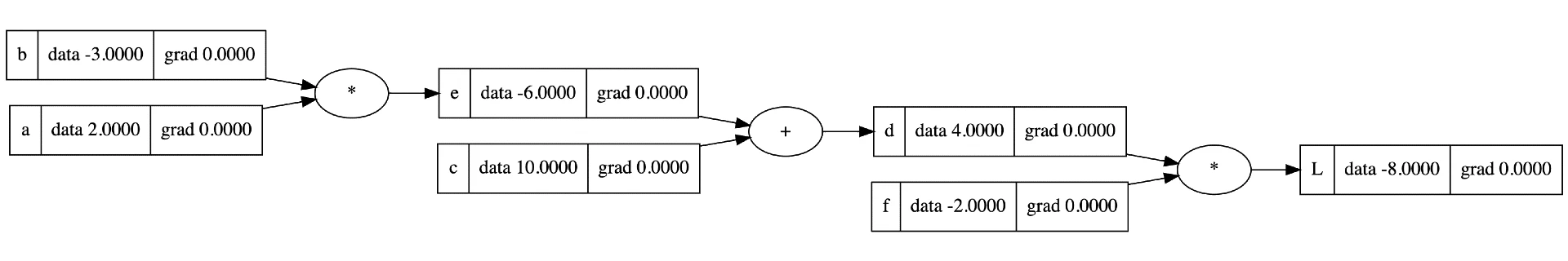
This image is a computation graph visual generated from Andrej Karpathy’s micrograd repo. Micrograd is a small scalar-based autograd engine written in Python. It in total is only a couple hundred lines of code, and I highly recommend anyone who hasn’t seen it to watch it.
Not too long ago, I started to build an autograd engine in Rust, but that fell into the large graveyard of dead projects. Recently I’ve been writing a lot of Go and have really appreciated the simplicity of the language and the speed of development, so decided to give it another go with Go (hehe).
I started implementing an engine that used matrices as its basic unit of operation and had hit a few bumps when it came to implementing the vector calc. That’s when I decided that, before I implemented it with matrices, I should first implement a Scalar version based on micrograd.
Go Micrograd Implementation#
The basic building block in go-micrograd is the Value struct. Let’s look at the code below:
type Value struct {
	Data float64
	prev []*Value
	op   string
}

// Constructor
func New(f float64) *Value {
	return &Value{Data: f}
}

// Add operation
func Add(a, b *Value) *Value {
	return &Value{
		Data: a.Data + b.Data,
		prev: []*Value{a, b},
		op:   "+",
	}
}

// Multiplication operation
func Mul(a, b *Value) *Value {
	return &Value{
		Data: a.Data * b.Data,
		prev: []*Value{a, b},
		op:   "*",
	}
}
We have a Value struct with two operators, Add and Mul. Each Value instance contains a float64 and metadata about previous operations.
// Example
func main() {
	a := New(2.0)
	b := New(-3.0)
	c := New(10.0)
	d := Add(Mul(a, b), c)

	d.DisplayGraph()
}
We’ll find here that when we construct a new Value via New(), the Value instance only contains .Data and has an empty .op and .prev. When we get a new Value via an operation, however, the new Value has the operation for .op and the previous operand Value instances. You can see how, from sequential operations, we end up forming a DAG of Value instances with .prev as the children.
Now what is this d.DisplayGraph method? In Andrej Karpathy’s tutorial, he uses a Python library to display a nice visual of the computation graph. The d.DisplayGraph method is something I wrote to print a text representation of the computation graph to the terminal.
❯ go run main.go
 4 {  + [-6 10] }
-------------------
-6 {  * [ 2 -3] }
10
-------------------
 2
-3
-------------------
We see that d evaluated to 4 and was the result of Add(-6, 10). We see that the -6 was the result of Mul(2, -3) which were a and b respectively.
Adding Backpropagation functionality#
To add backpropagation, we need to add the following fields to the Value struct:
type Value struct {
    // ...
	Grad     float64
	backward func()
}
The Grad field allows us to store the gradient of the Value and backward allows us to store a function that allows us to calculate the gradient of the children.
func Add(a, b *Value) *Value {
	out := &Value{
		Data: a.Data + b.Data,
		prev: []*Value{a, b},
		op:   "+",
	}
	out.backward = func() {
		a.Grad += out.Grad
		b.Grad += out.Grad
	}

	return out
}

func Mul(a, b *Value) *Value {
	out := &Value{
		Data: a.Data * b.Data,
		prev: []*Value{a, b},
		op:   "*",
	}
	out.backward = func() {
		a.Grad += b.Data * out.Grad
		b.Grad += a.Data * out.Grad
	}

	return out
}
We add a Backprop() method to the Value struct. It is very similar to Karpathy’s implementation in Python. It works by constructing a topological ordering of the Values and then calling .backward() on the reverse ordering.
func (v *Value) Backward() {
	topo := []*Value{}
	visited := map[*Value]bool{}

	topo = buildTopo(v, topo, visited)

	v.Grad = 1.0

	for i := len(topo) - 1; i >= 0; i-- {
		if len(topo[i].prev) != 0 {
			topo[i].backward()
		}
	}
}

func buildTopo(v *Value, topo []*Value, visited map[*Value]bool) []*Value {
	if !visited[v] {
		visited[v] = true
		for _, prev := range v.prev {
			topo = buildTopo(prev, topo, visited)
		}
		topo = append(topo, v)
	}
	return topo
}
Training the double(x) Model#
Let us train a network that mimics the double(x) function from earlier. This will consist of one weight as before. We use two new operations Pow() and Sub() which we haven’t covered but they’re very similar to the Mul() and Add() operations from before.
func main() {
	x := New(2)
	w := New(0.4) // pretend random init
	y := New(4)

	for k := 0; k < 6; k++ {

		// forward pass
		ypred := Mul(w, x)
		loss := Pow(Sub(ypred, y), New(2))

		// backward pass
		w.Grad = 0 // zero previous gradients
		loss.Backward()

		// update weights
		w.Data += -0.1 * w.Grad

		fmt.Printf("Iter: %2v, Loss: %.4v, w: %.4v\n",
            k, loss.Data, w.Data)
	}
}
This training loop does the forward, backward, and update steps 6 times.
❯ go run main.go
Iter:  0, Loss: 10.24, w: 1.68
Iter:  1, Loss: 0.4096, w: 1.936
Iter:  2, Loss: 0.01638, w: 1.987
Iter:  3, Loss: 0.0006554, w: 1.997
Iter:  4, Loss: 2.621e-05, w: 1.999
Iter:  5, Loss: 1.049e-06, w: 2
We can see that after only 6 iterations, it already found the correct value of w to minimize the loss.
If you’re curious, here is what the computation graph looks like after the first iteration and after the last. I changed the .DisplayGraph() to look a little nicer.
After the first iteration:
❯ go run main.go
data 10.2400 | grad 1.0000 | prev { Pow [-3.2 2] }
-----------------------------------------------------------
data -3.2000 | grad -6.4000 | prev { + [0.8 -4] }
data 2.0000 | grad -0.1741
-----------------------------------------------------------
data 0.8000 | grad -6.4000 | prev { * [1.68 2] }
data -4.0000 | grad -6.4000 | prev { * [4 -1] }
-----------------------------------------------------------
data 1.6800 | grad -12.8000
data 2.0000 | grad -2.5600
data 4.0000 | grad 6.4000
data -1.0000 | grad -25.6000
-----------------------------------------------------------
After the final iteration:
❯ go run main.go
data 0.0000 | grad 0.0000 | prev { Pow [-3.2768e-07 2] }
-----------------------------------------------------------
data -0.0000 | grad 0.0000 | prev { + [3.99999967232 -4] }
data 2.0000 | grad 0.0000
-----------------------------------------------------------
data 4.0000 | grad 0.0000 | prev { * [1.99999983616 2] }
data -4.0000 | grad 0.0000 | prev { * [4 -1] }
-----------------------------------------------------------
data 2.0000 | grad -0.0000
data 2.0000 | grad -5.3333
data 4.0000 | grad 8.0000
data -1.0000 | grad 0.0000
-----------------------------------------------------------
You can check out the github repo here for further implementation details. It contains a much larger model (41 parameters, 3 layers, with tanh activation functions) and the implementation details of the other operations.